Formula Help Please

[Kenja824]

I have a spreadsheet with a large bit of statistics on it. NFL Stats for quarterbacks with every game of their career. First game is on the top and each line below it is his next game's stats.

On another sheet I have formulas already that shows his totals for whatever amount of games I put in cell A1. For instance if I type "30" into A1 then the line of stats next to that will show the totals for the first 30 games of his career.

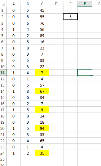
The image below is created for a simplified answer of course, but I was wondering how I can do this same thing but it would give the totals for the "last" 30 games of his career instead of the first 30. Reversing the order of the stats is not an option.

So for the image below, how would I write a formula that will add up the totals of only the last (however many as the number in cell E2) cells in column C that have a 1 in the same row in column A? (I colored the cells yellow to help clarify which cells I am talking about.)

with a 5 in E2 the formula would return 212
if E2 has 3 in it, the formula would return 138

Thanks ahead of time for any help.

 

[JG2828]

What is the current formula used to calculate the "first games"?

 

[IRstuff]

I would imagine that a non-VBA solution would involve count and offset functions

TTFN (ta ta for now)
I can do absolutely anything. I'm an expert!

https://www.youtube.com/watch?v=BKorP55Aqvg

faq731-376 forum1529 Entire Forum list

http://www.eng-tips.com/forumlist.cfm

 

[Kenja824]

unfortunately I dont have the file here at work. I will try to get my wife to log in and email it to me so I can see the formula I used. I cant remember what it was off the top of my head. lol

 

[Kenja824]

Here is the actual formula to one of the cells for stats.

=SUM(Brady!AA$1:INDEX(Brady!AA$1:AA$10000,MATCH($E2,Brady!$X:$X,0)))

Hmmmm, I thought I remembered using a sumif formula. lol I must have used that for another area and found this one to do this. Now that I have the file, I am attaching it as well so you can look at it.

Yes I know it would probably be better to use code instead of all formulas. I am just a lot more comfortable with formulas and I was hoping to finish this over one weekend.

You might notice scattered formulas and hilighting here and there as I was testing things and such.

 

[SkipVought]

Hey, Ken,

A picture doesn't cut it. I can't copy a picture of your data and paste it into a sheet.

Would like to use YOUR data so we can talk apples to apples.

Skip,

_{Just traded in my OLD subtlety...
for a NUance!}

 

[Kenja824]

Hey Skip:

Hah, caught you unexpected. lol Attached it in last message.


You will notice there are three tabs where I am drawing info from all of the players stats.
Compare has it where I can type in how many games I want to see totaled up, but that one only reads from top of the data going downward. Which is the first games of their careers. Which was my original need.

As it morphed, I wanted to see how they have done in the last so many games of their careers and havent found how to do that.

The other tabs allow me to look at how they played against specific opponents and the other lets me compare them for specific seasons.

I forgot my Revelations stuff at work I wanted to work on when home for the weekend and so I tackled this for the weekend instead. lol Almost got it done if not for this one formula kicking my butt.

 

[SkipVought]

Thanks for the upload.

I didn't see the sheet that you were originally referring to, so here's my table...
[pre]
A B C D E
1 1
1 2 5
0 3
0 4
1 5
0 6
1 7
0 8
[/pre]

Here are my formulae:
OffCellRef: =ADDRESS(COUNTA(A:A)-E2+1,1)
=SUMPRODUCT((OFFSET(INDIRECT(OffCellRef),0,0,E2,1)=1)*(OFFSET(INDIRECT(OffCellRef),0,2,E2,1)))

Notice I make a Named Range, OffCellRef that is relative to your E2 value.

Then the SUMPRODUCT (or you could use SUMIF) sums column C based on values in column A

Skip,

_{Just traded in my OLD subtlety...
for a NUance!}

 

[SkipVought]

I think that this is a better approach, just one formula:

=SUMPRODUCT((OFFSET($A$1,COUNTA(A:A)-E2+1,0,E2,1)=1)*(OFFSET($A$1,COUNTA(A:A)-E2+1,2,E2,1)))



Skip,

_{Just traded in my OLD subtlety...
for a NUance!}

 

[Kenja824]

Hey Skip

I am running into a problem with this I believe due to using COUNTA because where I gether the information is actually from a range of other formulas and so there are no empty cells. So when it finds the last one and counts whatever number back to get the address, it counts every cell because they all have formulas.

On the players actual tab I have a section on the left that is directly copied and pasted from NFL.com. Directly to the right of the pasted content, I have the same info pulled out of it using formulas. These formulas only display the games that fit certain criteria. If he started the game and if he attempted at least 15 passes. This helped me eliminate games when rookies and were thrust in to play a few snaps without preparing with the starters and such. But since there is a formula in every cell and just appearing as blank, the COUNTA still counts it.

I think I might be able to make your last formula work with Countif instead. I just need more time to work on it tonight as my lunch is over already. lol So tomorrow I will either be asking for more help or thanking you for your help. lol

 

[SkipVought]

The two COUNTA() column references need to be the same column in every sheet, that has something in each row that makes the count as it ought to be. That count is vital to locating the bottom of the range that you need to reference for the last x games.

Second, the third argument in the OFFSET Function will also need to change relative to that column, as it is the column offset.

Third, I’d name the cell containing the last x games to sum and use that Named Range in the fourth argument.

Skip,

_{Just traded in my OLD subtlety...
for a NUance!}

 

[SkipVought]

I am running into a problem with this I believe due to using COUNTA because where I gether the information is actually from a range of other formulas and so there are no empty cells.

Hmmmmm???

Looked at the Brady sheet and there are 287 rows in COUNTA(A:A) and that is the last row of 2017. That's exactly what we need!

Skip,

_{Just traded in my OLD subtlety...
for a NUance!}

 

[SkipVought]

So, I'm looking at the Brady sheet.

Column X, Heading G
Column AA, no heading, but looks like Wins 1 & Losses 0

So you're looking for sum of column X when there is a Win.

So for Brady I get 5651 for last 30 games

Last 30 rows...
[pre]
X Y Z AA AB
222 1 2016 1 W
223 1 2016 1 W
224 1 2016 1 W
225 1 2016 1 W
0 0 2016 0
226 1 2016 0 L
227 1 2016 1 W
228 1 2016 1 W
229 1 2016 1 W
230 1 2016 1 W
231 1 2016 1 W
232 1 2016 1 W
233 1 2016 1 W
234 1 2017 0 L
235 1 2017 1 W
236 1 2017 1 W
237 1 2017 0 L
238 1 2017 1 W
239 1 2017 1 W
240 1 2017 1 W
241 1 2017 1 W
0 0 2017 0
242 1 2017 1 W
243 1 2017 1 W
244 1 2017 1 W
245 1 2017 1 W
246 1 2017 0 L
247 1 2017 1 W
248 1 2017 1 W
249 1 2017 1 W
[/pre]

For that here's my formula with 30 hard coded, on the Season sheet in G2 for Brady in C2...
[tt]
G2: =SUMPRODUCT((OFFSET(INDIRECT($C2&"!"&"$A$1"),COUNTA(INDIRECT(C$2&"!"&"A:A"))-30,23,30,1))*(OFFSET(INDIRECT(C$2&"!"&"$A$1"),COUNTA(INDIRECT(C$2&"!"&"A:A"))-30,26,30,1)=1))
[/tt]

The first OFFSET is summing column X and the second OFFSET is condition =1.


Skip,

_{Just traded in my OLD subtlety...
for a NUance!}

 

[SkipVought]

You have this formula in column AK (GS)
[tt]
=IF($Y262=1,F262,[highlight #FCE94F]""[/highlight])
[/tt]

If you want to SUM in this column you can't have [highlight #FCE94F]""[/highlight].

Skip,

_{Just traded in my OLD subtlety...
for a NUance!}

 

[Kenja824]

In Brady's stats up above, you actually have his last 28 games as two of those games he did not play in. Those are the last 30 games for the team, but he only played in 28 of those. I would need to add up the last thirty games that have a 1 in column Y.

The problem I have is that code ..... =IF($Y262=1,F262,"") ........ is there trying to separate full games from partial games and missed games. A good one to look at is Winston as he misses quite a few games recently.

To my understanding, when you use the "" in a code, it makes the cell appear blank but its not actually a blank cell. But with a lot of functions I find it still works well. Just not with COUNTA I think. So I would need to find some other way to separate the missed games from the played games, or I need to find another way to sum up the totals.

To be honest, I have never known much about the "indirect" that your statement uses above, and though it is already being used in some cells in this file, I must have stolen the code and got lucky on adjusting it. lol I was just starting to understand how it works last night at 2:30 AM when I realized I just needed to go to bed. Today at work I looked it up at one point and it makes a lot more sense now.

Im wondering if I can use the MAX to find the cell with the largest value in column X to find his last game played. Then using the Sum(Offset(Indirect to simply sum up a range that is offset from that cell. In the offset where you place the number for row offset, and where you place the number for how many rows, I can link both to a cell like C2 in the sheet where I want the totals to come up. Just a thought at this point but I havent had a chance to play with it yet. God knows I am probably not explaining it clearly so forget this part of the post. lol

Waiting for lunch.... very.... impatiently.... lol

 

[Kenja824]

So this is what I came up with that seems like it will work.

=SUM(INDIRECT("Brady!y"&MATCH(MAX(Brady!X:X)-B1+1,Brady!X:X,0)&":y"&MATCH(MAX(Brady!X:X),Brady!X:X,0)))

(It seems to work so far)

It finds the max value in column Y and minuses cell B1 from it (plus 1) To find the row of the first game to be summed. It then finds the max value in Y and returns its row number. Then it returns the sum from the one row to the other on column X.

This ignores the games the player did not play in or bye weeks.

Understanding the "Indirect" really makes a difference. lol

Thanks for the help.

 

[SkipVought]

Okay, here's your workbook with ONE FORMULA that can be used across the table with the exception of your percentage calculations.

One caveat:
1) Insert a row above your table in sheet Compare and
2) in row 1 enter the Column Reference
3) the cell containing the last number of games is named [highlight #FCE94F]GAMES[/highlight]

Here is your formula...
[pre][tt]
[highlight #FCAF3E]AA[/highlight]
GAMES [highlight #FCE94F]25[/highlight] PLAYER WINS
[highlight #729FCF]BRADY[/highlight] =SUM(INDIRECT([highlight #729FCF]$C3[/highlight]&"!"&[highlight #E9B96E]D$1[/highlight]&MATCH(MAX(INDIRECT([highlight #729FCF]$C3[/highlight]&"!$X:$X"))-[highlight #FCE94F]GAMES[/highlight]+1,
INDIRECT([highlight #729FCF]$C3[/highlight]&"!$X:$X"),0)&":"&[highlight #E9B96E]D$1[/highlight]&MATCH(MAX(INDIRECT([highlight #729FCF]$C3[/highlight]&"!$X:$X")),INDIRECT([highlight #729FCF]$C3[/highlight]&"!$X:$X"),0)))
Brees 15
[/tt][/pre]


Skip,

_{Just traded in my OLD subtlety...
for a NUance!}