for Pi, Mxi, and Myi:
Lets first look at P, where P is the total force of the compression area.
From first principals Force = Stress x Area, which is some value or function x Area = Volume
From calculus to find the volume you need to do the double integral of a function, F(x,y) over finite areas, dA
That's all well and good right but what are the integral bounds and what is F(x,y)?
So our problem is a little tricky in that sense because:
1. The boundary is whatever the user defines the plate shape to be.
2. F(x,y) we really don't know other than that we know the stress distribution is linear.
Assumption 1: Stress varies Linearly
So given what we do know how can we go about performing that double integral, This is where Green's Theorem,
Link, comes in if we define the plate by piecewise linear segments with vertices defined in a counter-clockwise order we can apply Green's Theorem.
Assumption 2: the plate shape will be defined by linear segments with vertices defined in a counter-clockwise order.
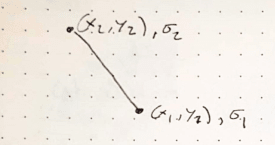
From Assumption 1 and 2 lets look at an arbitrary line segment defined by two points having stress,1 at point 1 and stress,2 at point 2:
Being an arbitrary line we now need some mathematically functions that define the line so that we actually have something to integrate, lets define the line using parametric equations in a time domain of 0 <= t <= 1:
x(t) = x,1 + t (x,2-x,1) - test: t=0, x(0)=x,1 and t=1, x(1)=x,1+ x,2 -x,1 = x,2
y(t) = y,1 + t (y,2-y,1)
sigma(t) = sigma,1 + t (sigma,2 - sigma,1) <--- Assumption 1: Stress is Linear
Now we have some math functions to have some fun with. Lets look at Green's Theorem:
Assumption 3:We are going to rotate the cross section/plate so that the stress always only varies in the Y direction.
using Assumption 3, Force = Stress * area => Stress = F(x,y) => F(x,y) * area, but now stress only varies in Y so F(x,y) now becomes F
")
and because we are now looking at an Arbitrary line F
= stress = sigma(t):
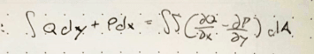
Integral Q dy + Integral P dx = dbl integral (dQ/dx - dP/dy) dA = dbl Integral F
dA = dbl Integral sigma(t) dA, note the dQ/dx and dP/dy are partial derivatives
since our function relies on Y lets try to find functions Q and P so that one of them drops out when we look at the partial derivatives:
Try:
Q = sigma(t)*x --> dQ/dx = sigma(t)
P = 0 --> dP/dy = 0
dQ/dx - dP/dy = sigma(t), which matches above so we can move forward now.
so now we have integral sigma(t) x dy + integral 0 dx, well integral of 0 is 0 so that piece drops off:
Integral sigma(t) x dy
We need to now substitute it to get everything in terms of variable t
remember from above: x(t) = x,1 + t(x,2-x,1)
for dy we know y(t)=y,1+t(y,2-y,1) so then for a small change in y we need a small change in t, dt:
dy/dt = (y,2-y,1) or dy = (y,2-y,1) dt
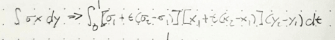
and substituting everything from above in we get:
Integral (sigma,1+t(sigma,2-sigma,1)) * (x,1+t(x,2-x,1)) * (y,2-y,1) dt
The bounds of this integral are now the time domain 0 to 1
You can use various tools to solve this integral symbolically, I've been using Maxima:
Link
So all of that gets us to a formula for P for an arbitrary line segment.
Formulas for Mx and My are found in a similar way:
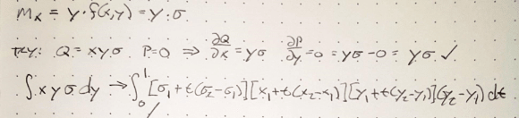
Knowing that Mx = Force * some y distance and force = stress * area
then Mx = dbl integral y * F(x,y) dA = dbl integral y*F
dA = dbl integral y*sigma(t) dA
Green's Theorem substitution:
Q = x y sigma(t) --> dQ/dx = y sigma(t)
P = 0 --> dP/dy = 0
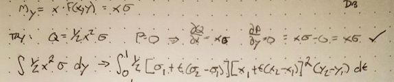
Knowing that My = Force * some distance x and Force = stress * area
then My = dbl integral x * F(x,y) dA = dbl integral x*F
dA = dbl integral x*sigma(t) dA
Green's Theorem substitution:
Q = 1/2 x^2 sigma(t) --> dQ/dx = x sigma(t)
P = 0 --> dP/dy = 0
Solving all of the above integrals will give you general formulas for P,Mx,My of an arbitrary line segment.
You'll notice though that point 1 of the segment needs to have a stress value, what happens if the stress region is only partly on an edge segment?
In this instance you need to break up the segment to fit within the integration bounds and create a new segment where the first point lies at the exact point of 0 stress.
Also of that work above was just for a line segment to get the total P, Mx, and My you sum all of the segment components for the entire stress boundary. one thing you may notice is that each integral has a (y,2-y,1) term so if Y is constant across a segment it's contribution to P, Mx and My is 0 so if programming this you could include a check and skip those segments to help improve computation time.
Edit:
So one thing which may not be immediately apparent is, what happens if your stress function F(x,y)=1?
Well the P integral becomes -> dbl integral 1 dA, which the volume of an object with unit height is equal to the Area of that object
From mechanics of materials the first moment of area or elastic section modulus is:
integral x dA or integral y dA, which should look pretty similar to the formulas we just derived above for My and Mx
Again from Mechanics of materials the second moment of area of Moment of Inertia is:
integral x^2 dA or integral y^2 dA, following the procedure above we could come up with Q and P functions for these and use Green's Theorem again to get an integral for an arbitrary line section.
So that is a long winded way to say if the stress function, F(x,y), is equal to 1, then the results of the integrals are just the geometric section properties of the shape you've defined by line segments.
For area you may be familiar with the "Shoelace" formula, our formula for P above with an F(x,y)=1 is actually the derivation for the "Shoelace" formula.
Link
My Personal Open Source Structural Applications:
Open Source Structural GitHub Group: