Heat Map Plot is Blocking data Behind it

dB_Field_con=dB_Field*(1e7/4/pi);% [A/m^2]
[Z,X] = meshgrid(x,z(2:length(z)));
figure1 = figure('units','normalized','outerposition',[0 0 0.5 0.5]);
axes1 = axes('Parent',figure1);
hold(axes1,'on');
s=surf(Z,X,dB_Field,'Parent',axes1,'LineStyle',':');
s.EdgeColor = [0.3 0.3 0.3];
title(['Magnetic Gradient dH (line ' txt ')'],'FontSize', 30)
ylabel({'(distance from magnet surface)';'Z[mm]'},'FontSize', 22)
xlabel({'X[mm]';'(distance on magnet surface)'},'FontSize', 22)
view(axes1,[0.100000000000001 90]);
grid(axes1,'on');
axis(axes1,'tight');
set(axes1,'DataAspectRatio',[1 1 1],'FontName','Times New Roman');
% 'FontSize',...
%     14
c=colorbar('peer',axes1);
colormap jet
c.Label.String = 'dH[T/m]';
%saveas(gcf,['contour gradient line ' line '.pdf']);

D=10e-9; %m
R=D/2;
Vp=4/3*pi*R^3;%m^3
rho=1.19e3; %kg/m^3
Ms=22e-3*(1e7/4/pi); %[T]to [A/m] - Saturation Magnetization (Ms)
IMS=4.04; %Initial Magnetic Susceptibility
mu0=1.256e-6; %Vs/Am
g=9.81; %m/s^2
Fm=mu0*Vp*Ms*dB_Field_con; %[N]
Fg=rho*Vp*g; %N
F_normalized=Fm/Fg; % one particle
% graphs


figure1 = figure('units','normalized','outerposition',[0 0 0.5 0.5]);
axes1 = axes('Parent',figure1);
hold(axes1,'on');
%s=surf(Z,X,F_normalized,'Parent',axes1,'LineStyle',':');

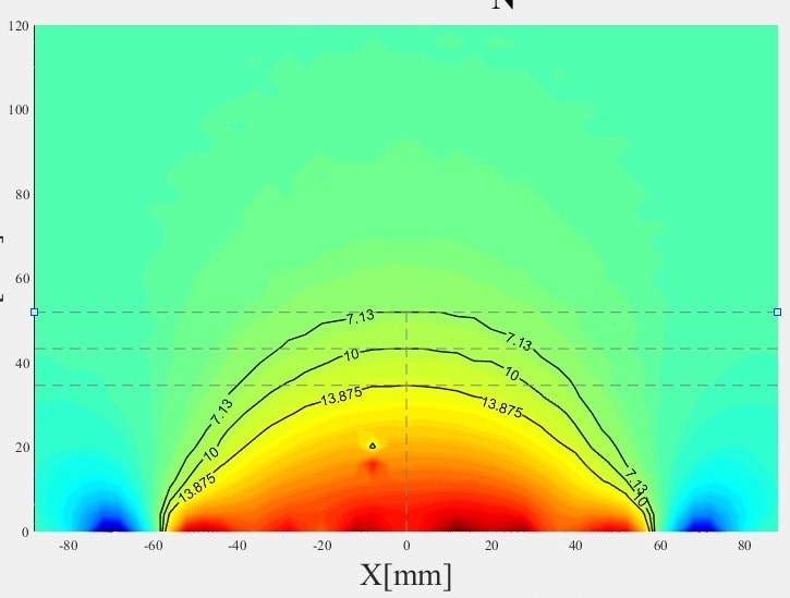
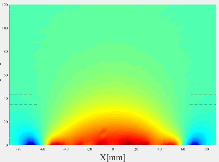
contour(Z,X,F_normalized,'LineWidth',1,'LevelStep',1,'Fill','on');
[c1,h1] = contour(Z,X,F_normalized,'LineWidth',1,'LineColor',[0 0 0],...
    'LevelList',[7.13 10 13.875]);
clabel(c1,h1);
plot([-88 88],[51.976 51.976],'--','Color',[0.5 0.5 0.5])
plot([-88 88],[43.3133 43.3133],'--','Color',[0.5 0.5 0.5])
plot([-88 88],[34.65 34.65],'--','Color',[0.5 0.5 0.5])
plot([0 0],[0 51.976],'--','Color',[0.5 0.5 0.5]);

s.EdgeColor = [0.3 0.3 0.3];
title(['Normalized Force F_{N} (line ' txt ')'],'FontSize', 30)
ylabel({'(distance from magnet surface)';'Z[mm]'},'FontSize', 22)
xlabel({'X[mm]';'(distance on magnet surface)'},'FontSize', 22)
view(axes1,[0.100000000000001 90]);
grid(axes1,'on');
axis(axes1,'tight');
set(axes1,'DataAspectRatio',[1 1 1],'FontName','Times New Roman');
% 'FontSize',...
%     14
c=colorbar('peer',axes1);
colormap jet
c.Label.String = 'F_{Normalized}';
%saveas(gcf,['contour normalized force line ' line '.pdf']);
% center
F_n_center=F_normalized(:,23);
[fitresult, gof] = createFit_260519(z(1:length(z)-1), F_n_center)