Conditional Formating - 2 conditions 1

[SBaugh]

I am trying to find some help on setting up a conditional formating that has 2 conditions that are true. The problem I am having is that I need certain cells to highlight per month (equal or greater than) and the other condition is the selection value that ultimately determines the color.

Example Spreadsheet:

https://docs.google.com/spreadsheet...ouid=104306274075149118717&rtpof=true&sd=true

Per this Formula, it highlights the entire row, not just the cells equal to or greater than the current month.

Is there any way to make this work or is there a different way I need to look at this? If VBA would allow this to work I am fine doing it like that as well, not sure how to write the code though.


Scott Baugh, CSWP
CAD Systems Manager
Dapco, INC

http://www.dapcoinc.com

"If it's not broke, Don't fix it!"

faq731-376

 

[3DDave]

What are the two condition? Can you attach the example file here?

 

[SBaugh]

There is a file in my original post.

The 2 conditions are the option selection in Column "E" and the month. If the current month is equal to or greater than and varying on the "E" column selection varies the color of the cell that falls under the equal or greater than months that of course has a value in the cell.

Scott Baugh, CSWP
CAD Systems Manager
Dapco, INC

http://www.dapcoinc.com

"If it's not broke, Don't fix it!"

faq731-376

 

[electricpete]

> There is a file in my original post.


Access denied.

I'm sure there is either a priority or an order to the conditions. I think the last condition would remain but may erase some of earlier conditions if they are trying to control the same formatting aspects. One way around it (besides changing order or priority) is to change different aspects of formatting... for example one condition changes the [highlight #EF2929]background color[/highlight] and the other changes the bold status so you can visually distinguish when [highlight #EF2929]both conditions[/highlight] are satisfied

=====================================
(2B)+(2B)' ?

 

[SBaugh]

Sorry about that, try this:

https://docs.google.com/spreadsheet...ouid=104306274075149118717&rtpof=true&sd=true

Scott Baugh, CSWP
CAD Systems Manager
Dapco, INC

http://www.dapcoinc.com

"If it's not broke, Don't fix it!"

faq731-376

 

[electricpete]

Thanks for the new sheet. I didn't get very far.

Here is an excel conditional formatting dialogue box with some things highlighted in yellow:

I wanted to mention a few things including the two things higlighted above:
[ul]
[li]1 - Rules are applied in the order listed. So the later rules that are true can overwrite the format of earlier rules that are true.[/li]
[li]2 - If you want the format of an earlier condition to stick, then check the box on the right "stop if true" so that it won't be overwritten.[/li]
[li]3 - As mentioned before, if you want to visually display the status of two different true conditions in the same cell, then they shouldn't change the same formatting attribute. (If both conditions are trying to change the background color then only one will display no matter what you do). So an alternative example use bold font for one condition and [highlight #EF2929]background color[/highlight] for the other so excel can display [highlight #EF2929]both[/highlight]. Example below highlights both odd numbers and numbers > 2 and you can tell cell B3 meets both:[/li]
[/ul]

I'm not sure if that answers your specific question. If not, what particular cell are you concerned about and what do you want it to show?

=====================================
(2B)+(2B)' ?

 

[SBaugh]

Wow, thanks! For as many years as I have been using Excel I never knew that's how Conditional formatting was going through it or how to stop it. - Thanks!

I will try and explain this again. My manager has this spreadsheet that he uses to track all the active projects and the shop hours.

Since Sept is the active month then he highlights all the hours per the project status manually. If "rebuilt" it's blue, if "New" it's red. (His legend is at the top)

All I am trying to do is automatically highlight the cells per the active month (1 condition) or if there are values in the up and coming months those are highlighted as well (greater than) Per the Project status (2nd condition). Since there are 6 different options I assume that I will have to write a conditional format for each type, since the project status is more dynamic than the month.

Anything less than the current month is that gradient background.

The problem is I cannot figure out to use conditional formatting to achieve this. - does that make sense? or help you to help me?

Scott Baugh, CSWP
CAD Systems Manager
Dapco, INC

http://www.dapcoinc.com

"If it's not broke, Don't fix it!"

faq731-376

 

[electricpete]

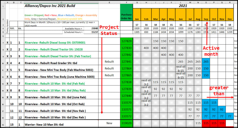
Since Sept is the active month then he highlights all the hours per the project status manually. If "rebuilt" it's blue, if "New" it's red. (His legend is at the top)

All I am trying to do is automatically highlight the cells per the active month (1 condition) or if there are values in the up and coming months those are highlighted as well (greater than) Per the Project status (2nd condition). Since there are 6 different options I assume that I will have to write a conditional format for each type, since the project status is more dynamic than the month.

Anything less than the current month is that gradient background.

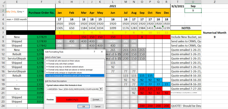
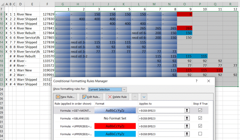
Below / attached I tried to implement this using the first several rows of your data (I discarded all the original formatting / conditional-formatting because I didn't want to figure it out). I could not figure out what you wanted different between current month and future months, so I treated current and future months the same.

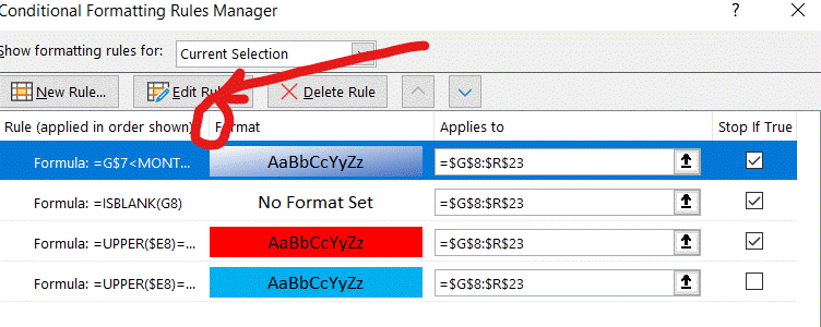
I created four conditional format rules in the range $G$8:$R$23 (The ULHC, G8, for that range is significant because it gives context to the formulas). Here are the four rules:
[ul]
[li]1st condition: =G$7<MONTH(TODAY()) [format graded shading] STOP IF TRUE[/li]
[li]2nd condition: =ISBLANK(G8) [format none] STOP IF TRUE[/li]
[li]3rd condition: =UPPER($E8)="NEW" [format red] [stop is optional here][/li]
[li]4th condition: =UPPER($E8)="REBUILT" [format blue][/li]
[/ul]
Note that the STOP IF TRUE on the 1st and 2nd conditions simplified the formula for the 3rd and 4th conditions:
[ul]
[li]The 3rd and 4th conditions don't need to check that date is this month or greater, because of earlier 1st condition stop if true.[/li]
[li]The 3rd and 4th conditions don't need to check if cell has anything in it, because of the earlier 2nd condition stop if true.[/li]
[/ul]

That recreates the screenshot and colors in the spreadsheet for this portion of the spreadsheet.... which I'm assuming were originally added by hand without conditional formatting (if they were originally created by conditional formatting then I just recreated the same thing that you already had).

Since there are 6 different options I assume that I will have to write a conditional format for each type...

I think you're saying there are 4 more options beyond New and Rebuilt that need their own color. If so then I think you're right about that... I don't see any way to get around creating a conditional formatting rule for each option (excluding maybe some vba trickery)

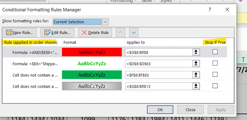
EDIT - In case anyone is having a hard time following this. Here's what my spreadsheet ends up doing (my interpretation of what op requested, whether right or wrong):
[ul]
[li]1 - any cell (empty or not) in a column whose month is less than current month is gradient light blue.[/li]
[li]2 - any non-empty cell in a column whose month is current month or later is either[/li]

[li]2A - Red if "New" in column E[/li]

[li]or[/li]​

[li]2B - Blue if "Rebuilt" in column E[/li]​

[/ul]
===============================

=====================================
(2B)+(2B)' ?

 

[SkipVought]

@electricpete, I wasn't criticizing you at all. It was directed @ the OP. You are on the right track.

But then I read further and saw he did eventually explain his specs.



Skip,

_{Just traded in my OLD subtlety...
for a NUance!}

 

[electricpete]

No problem. I added the specification for my particular spreadsheet to the end of my last post just in case it helps anyone figure out what I was trying to do.
=====================================
(2B)+(2B)' ?

 

[IRstuff]

Seems like the posted sheet is missing a referenced tab called "Data Info"

The rule in G8:R8 shows =AND($E$8="New",$Z$8=$U$2,INDEX(G8:R8,COUNTA(G8:R8))) but are $E$8 and $Z$8, since those are absolute references to a single cell, as opposed to the relative cell, i.e., $E8 and $Z8 instead?



TTFN (ta ta for now)
I can do absolutely anything. I'm an expert!

https://www.youtube.com/watch?v=BKorP55Aqvg

faq731-376 forum1529 Entire Forum list

http://www.eng-tips.com/forumlist.cfm

 

[electricpete]

> The rule in G8:R8 shows =AND($E$8="New",$Z$8=$U$2,INDEX(G8:R8,COUNTA(G8:R8))) but are $E$8 and $Z$8, since those are absolute references to a single cell, as opposed to the relative cell, i.e., $E8 and $Z8 instead?

That equation is quite a mess. If you can figure out how it's supposed to work, then you're a better man than me. Changing $E$8 to $E8 is logical, but $Z$8=$U$2 is problematic no matter what you do with it. As written it's useless because it's always true due to the formula in $Z$8 "=U2". But if you change it to $Z8=$U$2 it's still not going to work because there is nothing in the cells below Z8 (Z9, Z10 etc).

And this whole thing is within an AND that has 3 logical arguments, the last of which is INDEX(G8:R8,COUNTA(G8:R8)).... returning the contents of a cell within G8:R8 (or the relative shifted version of it) located at the position within that range indexed by the total number of non-empty entries in that range (and the contents of that cell will be treated as a boolean argument). I gather this last argument is an attempt to check for empty cells but it will not work. When I do a test of this approach using a formula AND(1,A1) that test returns TRUE whether A1 is empty or not (it only returns false if A1 contains 0 or FALSE). Given that the example data contains no data which is FALSE or a numeric 0, this argument will always return true to that argument within the and() function. If intent is to check for empty cells, he could've simply used isblank.

I gave up on trying to piece together the logic from those formulas or suggest correction. Op stated he can't figure out how to do what he wants with conditional formatting, but he described in words and manually-colored screenshots what he wanted to do. I suggested an approach above which I believe is fairly simple (only one logical test per rule) in comparison to this convoluted formula.

=====================================
(2B)+(2B)' ?

 

[SBaugh]

That is Amazing! I would have never figured that out. Works great!

I don't totally understand exactly how it works. Conditional formatting is not easy for me to understand anyway, but it's great having you experts out there willing to help out.

Thank you so much for this.

The only question I have now is once we go to the next month how will it know to switch to the next column?

Scott Baugh, CSWP
CAD Systems Manager
Dapco, INC

http://www.dapcoinc.com

"If it's not broke, Don't fix it!"

faq731-376

 

[electricpete]

The only question I have now is once we go to the next month how will it know to switch to the next column?

1st condition: =G$7<MONTH(TODAY()) [format graded shading] STOP IF TRUE

Today() updates itself each day
MONTH(TODAY()) will update itself each month.

> I don't totally understand exactly how it works.

I realize it all depends on your exposure to these things.
You are already familiar with boolean logic.
The only tricky thing about my implementation is that it relies on sequential application of rules (so you'll have to run through the rules sequentially in your mind to figure out how it will work).
In my mind that makes it simpler. Maybe that's in the eye of the beholder.

If you wanted to do the same thing without relying on sequential application of rules (no STOP IF TRUE), then you could do as follows
[ul]
[li]1st condition: =G$7<MONTH(TODAY()) [format graded shading][/li]
[li]2nd condition: (no longer needed)[/li]
[li]Revised 3rd condition: =AND(UPPER($E8)="NEW", G$7>=MONTH(TODAY()), NOT(ISBLANK(G8)) [format red][/li]
[li]Revised 4th condition: =AND(UPPER($E8)="REBUILT" , G$7>=MONTH(TODAY()), NOT(ISBLANK(G8)) [format blue][/li]
[/ul]
This revised non-sequential version is more complicated imo... it involves 7 logical arguments where my original sequential version only required 4 logical arguments. Plus the revised version jumbles those logical arguments into two 3-input and() functions where someone (me anyway) is more likely to make a mistake in a long formula. And if you are adding more options beyond "new" and "rebuilt", then each additional option would require another 3-input and() function.


=====================================
(2B)+(2B)' ?

 

[SBaugh]

Your logic makes total sense and it made it much easier to set up the other drop-down menu option colors. Thank you!

What totally blows me away is when you add something to the conditional formatting, apply it, and have to go back in a change the formula because it goes from E8 to E1057846 or something, just crazy.

Thanks for all your help, its Truly appreciated!

Scott Baugh, CSWP
CAD Systems Manager
Dapco, INC

http://www.dapcoinc.com

"If it's not broke, Don't fix it!"

faq731-376

 

[3DDave]

I agree - very frustrating. Under the hood I think that conditional formatting is yet another macro language that doesn't behave exactly the same as in-cell formulas. When a different cell is chosen from the one where the conditional formatting was first created it calculates new offsets from the new cell, which might be above or to the right and would, for an in-cell formula, cause an error, instead they roll like an odometer and it counts back from the maximum number.

I'm betting on summer interns given a task that come up with this stuff. Instead of building a core functionality that is universal and consistent they build independent modules, so they all work a little different.

 

[electricpete]

To be sure, there is a lot of funkiness when trying to edit the format condition equation. One thing I notice is that if I click from the equation onto the spreadsheet (to identify an address) and then use arrow keys to try to move my cursor within the formula, excel is moving my cursor in the spreadsheet (cell selection) rather than moving my cursor within the formula.

Also, it would be nice if I could drag the stinkin’ vertical line between “rule” and “format” column headings to show the entire rules, but nooooo.....

Also the "applies to" field in the above dialgue box will accept a named range but it won't remember it as a named range (it just remembers it as an address... which won't be adjusted if I change my named range later). So we can't enter the range as a named range and expect to be able to tweak the bottom / right edges of the named range later (we wouldn't want to tweak the upper/left edges of the named range anyway, due to impact on formulas). As an aside it occurs to me it might have been more elegant to enter the range as the entire columns =$G:$R and then exclude the starting rows by adding a condition up front =row(G1)<8 [format none] STOP IF TRUE. Since the range would then start with G1, that would also require you to subtract 7 from all the relative row references (numbers without a $ in front) in all my previous formulas that were based on a range starting in G8 (i.e. change $E8 to $E1 and G8 to G1)

Going back to what might be tricky about this example....
IR stuff made a comment about op's error in cell relative and absolute references (which maybe I shouldn’t have downplayed).
I think we all know how relative and absolute references work when copying cell formulas, but maybe it's not as intuitive for conditional formatting.
So maybe it's useful to imagine that the formula entered for conditional formatting of a range is entered into the upper left corner cell of that range and then copied to the other cells of the range. The absolute/relative references translate in the same way that they do for copying.

=====================================
(2B)+(2B)' ?

 

[SkipVought]

So maybe it's useful to imagine that the formula entered for conditional formatting of a range is entered into the upper left corner cell of that range and then copied to the other cells of the range. The absolute/relative references translate in the same way that they do for copying.

That's GOLD! It is the key to CF formulae construction.

Skip,

_{Just traded in my OLD subtlety...
for a NUance!}

 

[SBaugh]

electricpete - Question since I know I cannot suppress a conditional format until I want to use it. Can the conditional format that changes the Background to a gray gradient, go by the month, day, and year? If so how would I set that up?

Currently its setup:
=G$7<MONTH(TODAY())

G7 = 1

Scott Baugh, CSWP
CAD Systems Manager
Dapco, INC

http://www.dapcoinc.com

"If it's not broke, Don't fix it!"

faq731-376

 

[SkipVought]

Where in that row is day and year?

Or are you referring to TODAY()?

What specification for month, day, year and format?

Skip,

_{Just traded in my OLD subtlety...
for a NUance!}