I can think of 2 ways to do this.
I am not an Abaqus user, so I don’t know if the second solution is possible in this code, but the first should be.
Solution 1:
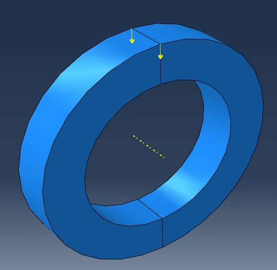
Under the assumption that the loads are axisymmetric, you could model a single segment of the solid over some theta angle. The angle is somewhat unimportant and will be governed more by the required mesh density in the axial and radial directions. Let’s assume you mesh a 1-degree segment (with 3D solid elements). The mesh should be a rotational sweep of the arc of the segment, such that you finish with the same pattern of nodes on side 1 of the segment as side 2 of the segment (these are the sides that would connect to the next segment if it were there).
With the segment meshed, define a cylindrical coordinate system for the nodes on both side 1 and side 2 boundaries. The radial, azimuth and axial directions of this coordinate system should be consistent with the rotational symmetry of the problem.
The simplest thing now is to define the analysis coordinate system (i.e. the coordinate system in which the displacement solution will be computed) of all the nodes as this cylindrical coordinate system, but strictly speaking, only the nodes on the “side” boundaries need be in this cylindrical coordinate system. You can also define the definition coordinate system (i.e. the system in which the node X,Y,Z positions are defined) as the cylindrical coordinate system, but this is a matter or preference. It can be useful to check all nodes on the perimeter have the same radius, for example.
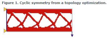
Now define a constraint equation between each of the nodes on side 1 and their counterpart on side 2. This constraint equation enforces axisymmetric behaviour and requires the loads to be symmetric (i.e. only harmonic 0 may be studied). The constraint in the radial and axial directions defines that a node on side 1 will follow the same radial (axial) displacement as side 2 (or the other way around if you prefer, the dependent/independent order is unimportant). The constraint in the azimuth direction is the opposite, i.e. it is defined to say that any azimuthal movement of a node on side 1 is in the opposite azimuthal direction to its counterpart on side 2. This is similar to a symmetric boundary condition, except the constraint is not to ground, it is to the other side of the segment.
Define the topology optimization task in the same way as for any 3D solid model (the model really is a 3D solid model, you just constrain it to behave with axisymmetry).
Solution 2:
Topology optimization consists in assigning a material property to each individual element in the design region. If the software does not allow this to happen via its automatic interface, then define a unique material entry for each element and assign the design optimization task with one design variable per element. The link between material Young’s modulus and density is made via design to property links, one linear, one with a power law equation. Basically, you do the work manually. With a good text editor, or sometimes Excel can be a help here, you can prepare these data easily, at least this is the case for MSC Nastran, where the topology optimization task is possible with this “manual” configuration on axisymmetric elements (CTRIAX6 or CQUADX).
DG